This project currently has two software available to researchers in the field of multicollinearity and two-predictor suppressor effects: the Suppression simulator (Supsim), and the Suppression calculator (Supcalc).

Suppression Simulator (Supsim)

Download Users Guide for Supsim

Supsim is a computerized algorithm that enables users to easily generate numerous random, two-predictor models (RTM's) that some of them are affected by two-predictor suppressor effects while others are not. It is a specialized software made available as a web-based "JavaScript" application through this website (available here). A command-line "Python package" version of this software will also be releasaed soon. By specifying a number of parameters and running Supsim, users will be able to generate numerous series of random data vectors $x_1$, $x_2$, and $y$ in a way that regressing $y$ on both $x_1$ and $x_2$ by using each of the randomly generated datasets leads to numerous situations with or without suppression. The web-based "Supsim" also allows investigators to produce 3D scatterplots of these simulated RTM's.

The core idea of Supsim is to facilitate the study of two-predictor suppressor effects by generating numerous random functions (i.e., $y_o = f(x_1, x_2)$) and inserting errors into the outputs of those functions and then fitting OLS regression surfaces to the resulting noisy data ($y$). Figure 1 illustrates the RTM generation process step by step.

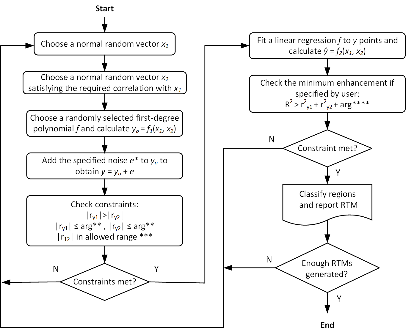
Figure 1: Flowchart of the Iterative Process of Generating RTM's

*: $e$ is a distribution of errors of the same length as $y_o$ (or original $y$), while mean and standard deviation of "$e$" is determined arbitrarily by the user as a proportion of mean and standard deviation of $y_o$. $e$ enables users to control the fit levels of the RTM's.

**: arguments (or arg's) are arbitrarily selected by the users to limit the magnitude of $r_{y1}$ and $r_{y2}$. By using arg's, users control the amount of $Cor(y,X1)$ and $Cor(y,x2)$.

***: There are two kinds of "allowed range" for $r_{12}$: first, the default allowed range is defined by $(r_{y1}.r_{y2}) - \sqrt{(1-r_{y1}^2).(1-r_{y2}^2)} \leq r_{12} \leq (r_{y1}.r_{y2}) + \sqrt{(1-r_{y1}^2).(1-r_{y2}^2)}$; Second, users are allowed to further limit the magnitude of $r_{12}$ by selecting an arbitrary range between 0 and 1.

****: arg's about the amount of $R^2$ enhancement enable users to arbitrarily control the levels of $R^2$ enhancement by selecting a proportion between 0 and 1. Leaving enhancement not specified, the algorithm generates all kinds of RTM's falling within suppression and redundancy regions, while selecting an enhancement proportion makes Supsim to generate only those kinds of RTM's that fall within enhancement regions. User's should be aware that when they specify a high proportion of enhancement (i.e. near 1), in fact they request the algorithm to produce RTM's with the highest fit levels (near 1), therefore they have to select the lowest $e$ magnitude (i.e. near 0) if their commands are to be feasible. User's also should be aware that in order for the $R^2$ enhancement to be close to 1, both $r_{y1}$ and $r_{y2}$ need to be close to 0 (and therefore, the value of $r_{y1}^2+r_{y2}^2$ would be close to 0 as a function), because according to inequality of $R^2> r_{y1}^2+ r_{y2}^2$ that always holds in enhancement situations the $R^2$ enhancement is defined as follows: $enhancement = R^2 - (r_{y1}^2+r_{y2}^2)$.

---

It should be noted that when designing the algorithm of Supsim the authors noticed that one of the challenging constraints to meet was the specified amount of correlation between $x_1$ and $x_2$. They observed that satisfying this constraint requires an exhaustive search over a very large space of all possible RTMs which is not feasible in a reasonable time. Therefore, a prerequisite step is to randomly produce normal distributions of $x_1$ and $x_2$ vectors so that they show a random amount of correlation with each other ($r_{12}$) before using $x_1$ and $x_2$ vectors in random functions of $y_o$. Generating random numbers by using the Whuber's method (Whuber, 2017), the authors succeed to solve the problem of producing correlated, random, normal vectors $x_1$ and $x_2$ and to speed up the simulation process.

According to Whuber's method (2017), the algorithm shown in Figure 1 first chooses a normal random vector $a$ with the same length, mean, and standard deviation as $x_1$ and then applies a transformation to it to calculate $b$ in a way that the correlation between $b$ and $x_1$ is set to the desired amount ($r$). Such a transformation is described in Equation (1) where $d$ is the vector of residuals resulted from regressing $a$ on $x_1$, $\sigma_d$ represents the standard deviation of $d$, and $\sigma_{x_1}$ represents the standard deviation of $x_1$. It should be noted that such a transformation changes the initial distribution properties in $b$ vector. Therefore, in order to return $b$ to a mean and a standard deviation equal to $x_1$, $x_2 = m.b+n$ is used as the final random, correlated, normal vector, where $m = \sigma_{x_1}/\sigma_b$ and $n = \mu_{x_1}-m.\mu_b$.

$$ b = r.\sigma_d.x_1 + d.\sigma_{x_1}.\sqrt{1-r^2} $$

Getting started with Supsim

Before running Supsim, users are asked to fill in the parameter boxes. These parameters help determine the desired characteristics of RTM's to be generated and provide users with a wide range of flexibility and control over RTM production process. The parameter boxes are defined as follows:

1- Size: Specifying an "integer", determines a "sample size" for $x_1$, $x_2$, and $y$ vectors.

2- Count: Specifying an "integer", determines the "number of RTM's" to be simulated.

3- Seed: Specifying a "value", determines a "seed" for the random number generator which is needed for "reproducibility" or "replicability". For example, when the users select the seed number of "1" to produce 50 RTM's, any time in the future when they again use seed = 1 and count = 50, Supsim reproduces exactly the same random vectors $x_1$, $x_2$, and $y$ as they had been generated at the first time.

4- Mean: Specifying a "value", determines "means" of the normal distributions of the two predictors $x_1$ and $x_2$.

5- SD: Specifying a "value", determines "SD's" of the normal distributions of the two predictors $x_1$ and $x_2$.

6- Noise: Specifying a "coefficient", determines a coefficient to be multiplied by both "means" and "SD's" of the original $y$'s (or $y_o$'s) to determine both means and SD's of the noise distribution to be used in generating $y$ vectors. As mentioned above, mean and standard deviation of $e$ vector or the noise is determined arbitrarily by the user as a proportion of mean and standard deviation of $y_o$. $e$ or noise level enables users to control the fit levels of the RTM's.

7- $r_{y1}$: Specifying a "value" (between 0 and 1), determines the maximum absolute value allowed for $r_{y1}$.

8- $r_{y2}$: Specifying a "value" (between 0 and 1), determines the maximum absolute value allowed for $r_{y2}$.

9- $r_{12}$: Specifying a "range", determines the minimum and the maximum absolute values allowed for $r_{12}$ (both of them between 0 and 1).

10- $R^2$ enhancement: Leaving "enhancement" not specified, the command prints RTM's falling within all regions with or without suppression. While, specifying an enhancement value (a proportion between 0 and 1), the command prints only those RTM's falling within enhancement regions which in turn each of the RTM's show at least "the specified value" or greater values of "$R^2$ enhancement".

11- Fraction: Specifying a "proportion" (between 0 and 1), determines a specific proportion of the generated RTM population to be randomly selected as "RTM sample" to be printed in the output Excel file. For example, if the user types "1" in the Fraction box, the entire data vectors (100%) related to all of the generated RTM's will be printed in output Excel file and by clicking "SAVE RTM's" the output Excel file will be downloaded and saved on the computer drives. If the user types 0.5 in the Fraction box, the data vectors for a randomly selected 50% of the generated RTM's will be saved in the output Excel file.

The Possibility of Selecting Model Parameters $R^2$, $\beta_{x_1}$, or $\beta_{x_2}$ to be Plotted on 2D Scatter Charts

Once the production process is completed, Supsim shows the position of the entire model parameters including the values of $R^2$, $\beta_{x_1}$, and $\beta_{x_2}$ coefficients for all the generated RTM's as differently colored dots on 2D scatter charts. The 2D scatter charts classify each of the RTM's to different suppression and non-suppression regions by comparing its properties with the definitions of each region presented by Friedman and Wall (Friedman and Wall, 2005). For example, all the RTM's falling within Region II redundancy on the regular graph show two similar characteristics: all of them are classified as a non-suppression situation (i.e., a redundancy region), $r_{y1}$ and $r_{y2}$ for all of those RTM's show similar signs which is characteristic of Friedman and Wall's regular graph. As another instance, all the RTM's falling within Region III suppression on reverse graph, show two similar features: all of them are negative suppression situations, $r_{y1}$ and $r_{y2}$ for all of those RTM's show opposite signs which is characteristic of Friedman and Wall's reverse graph. Each differently colored dots on the 2D scatter charts represents $R^2$, $\beta_{x_1}$, or $\beta_{x_2}$ coefficients, and a color guide is presented at the right side of each 2D scatter chart. By clicking the title of the model parameters presented in the right-side color-guide, users can hide dots related to that parameter from the 2D chart to see the locations of the remaining parameters separately on the chart. For example, if users want to see $R^2$ positions of all the generated RTM's separately on the 2D scatter chart, they can click the title of $\beta_{x_1}$ (Blue dots) and $\beta_{x_2}$ (green dots) parameters on the color guide to hide them.

The Possibility of Searching and locating RTM's with the greatest or the smallest values of $r_{y1}^2+r_{y2}^2$ on 2D Scatter Charts

Another useful possibility of the web-based JavaScript version of Supsim is its search buttons that enable users to rank and locate the first through the last RTM's with the greatest through the smallest values of $r_{y1}^2+r_{y2}^2$ on the 2D scatter charts. According to authors' experience RTM's with the greatest or the smallest values of $r_{y1}^2+r_{y2}^2$ are especially useful for case studies on unique suppression situations, and they are full of insight about the mechanisms causing suppression situations. Once the RTM production has finished and dots representing model parameters appeared on 2D scatter charts, buttons related to "Mark RTM Rank" under each scatter chart become active. Clicking "NEXT RANK" button at the right side will mark the first RTM with the greatest value of $r_{y1}^2 + r_{y2}^2$ and clicking "PREVIOUS RANK" button at the left side will mark the first RTM with the smallest value of $r_{y1}^2 + r_{y2}^2$. Users can successively click these two buttons to find 1st, 2nd, 3rd, …, nth ranks of $r_{y1}^2+ r_{y2}^2$ values in the generated RTM's.

Plotting each selected RTM in a 3D scatterplot

Although the entire data vectors $x_1$, $x_2$, and $y$ for each given "Fraction" are exported into an output Excel file so that the users can easily use them in drawing 3D scatterplots by using commercially available, specialized, software such as "NCSS" and "MATLAB", for users' convenience the web-based JavaScript version of Supsim can show the 3D scatterplots for each selected RTM by using the Plotly library. To see the 3D scatterplot of each selected RTM, the user should first select one of the colored dots on 2D scatter charts and click it to make Supsim open a new tab in the upper left corner of the website that when clicked on a new page would open that shows the 3D scatterplot of that selected RTM. An interactive feature of the 2D scatter charts is that when the user moves the mouse cursor and points to each particular colored dot (representing each particular RTM), a box pops up that shows $R^2$, $\beta_{x_1}$, $\beta_{x_2}$, and $r_{12}$ values for that given RTM. This important feature enables users to select RTM's with the desired properties among thousands of RTM's.

Download Users Guide for Supsim: Download Users Guide for Supsim

2- Suppression Calculator (Supcalc)

Download the Excel file of Supcalc: supcalc

Friedman and Wall (2005) have published an interesting work on two-predictor suppressor effects in which they introduce a useful application that plots $R^2$, $\beta_1$, and $\beta_2$ against $r_{12}$ values. Their application holds $r_{y1}$ and $r_{y2}$ constant and lets $r_{12}$ vary over its possible limit (see Figure 1 captions above for a detailed description about the allowed range of $r_{12}$) and then calculates and plots the entire variations in $R^2$, $\beta_1$, and $\beta_2$ as a function of variation in $r_{12}$. Graphical views generated by Friedman and Wall's creative application should be regarded as an important and seminal contribution to our understanding of two-predictor suppressor effects. We believe that Friedman and Wall's approach can be further extended to include more comprehensive inputs and outputs to create incredibly useful new insights into a full range of suppression situations (read our manuscripts for more details). the suppression calculator or supcalc is an extended non-graphical version of Friedman and Wall's application that receives arbitrary $r_{y1}$, $r_{y2}$ and $n$ values as input and calculates $R^2$, $\beta_{x1}$, $\beta_{x2}$, semipartial correlation and squared semipartial correlation of $x_2$ with $y$, the statistical control part ($SCP$), the collinearity-dependent part in both $\beta_{x1}$ ($CDPB1$) and $\beta_{x2}$ ($CDPB2$), the standard errors ($SE's$) of both $\beta_{x1}$ and $\beta_{x2}$, the collinearity ratios including $\gamma$ and $2\gamma/(1+\gamma^2)$, and the lower limit as well as the upper limit of $r_{12}$ as outputs (For more details about new outputs calculated by Supcalc please read our manuscript here). Interested readers can download the Excel file of Supcalc